Now that we have defined the entire model, we can start training the neural network. The idea of each step is to take one batch and predict the next position for each of the agents and positions. The result is then compared to the target values through the associated loss function we defined earlier.

Training

for e in range(NUM_EPOCHS):
    # Assign the learning rate (decayed acc. to the epoch number)
    lstm.sess.run(tf.assign(lstm.lr, lstm.learning_rate * (DECAY_RATE ** e)))
    # Reset the pointers in the data loader object
    pointer = data_tools.reset_batch_pointer()
    # Get the initial cell state of the LSTM
    state = lstm.sess.run(lstm.initial_state)
    
    # For each batch in this epoch
    for b in range(num_batches):
        start = time.time()
        # Get the source and target data of the current batch
        # x has the source data, y has the target data
        x, y, pointer = data_tools.next_batch(
            loaded_data, pointer, BATCH_SIZE, SEQUENCE_LENGTH)
        x = np.array(x)
        y = np.array(y)

        # Feed the source, target data and the initial LSTM state to the model
        feed = {
            lstm.input_data: x[:, :, 1:],
            lstm.target_data: y[:, :, 1:],
            lstm.initial_state: state
        }
        # Fetch the loss of the model on this batch,
        # the final LSTM state from the session
        train_loss, state, _ = lstm.sess.run(
            [lstm.cost, lstm.final_state, lstm.train_op], feed)
        # Toc
        end = time.time()

        cur_time = end - start
        step = e * num_batches + b
        
        avg_time += cur_time
        avg_loss += train_loss
        
        # Print epoch, batch, loss and time taken
        if (step%99) == 0:
            print(
                "{}/{} (epoch {}), train_loss = {:.3f}, time/batch = {:.3f}"
                .format(
                    step,
                    NUM_EPOCHS * num_batches,
                    e,
                    avg_loss/99.0, avg_time/99.0))
            
            avg_time = 0
            avg_loss = 0

os.makedirs(SAVE_PATH, exist_ok=True)
# Save parameters after the network is trained
lstm.save_json(os.path.join(SAVE_PATH, "params.json"))

Inference

After training is complete, we can start using it and infer the positions of agents in a never seen before data. When predicting trajectories of this type we assume that the agents observed have already walked for some time and we have the associated observed annotations. Thus, we “preload” the LSTM with the manner of walking of a particualr agent. Thus, we condition the associated predictions to the manner of walking, direction and behaviour of a considered agent. In addition we set the batch size to 1 and load the never seen before data set.

We sample from the predicted 2D Gaussian distribution in the following way:

def sample_2d_normal(o_mux, o_muy, o_sx, o_sy, o_corr):
  '''
  Function that samples from a multivariate Gaussian
  That has the statistics computed by the network.
  '''
  mean = [o_mux[0][0], o_muy[0][0]]
  # Extract covariance matrix
  cov = [[o_sx[0][0]*o_sx[0][0], o_corr[0][0]*o_sx[0][0]*o_sy[0][0]], [o_corr[0][0]*o_sx[0][0]*o_sy[0][0], o_sy[0][0]*o_sy[0][0]]]
  # Sample a point from the multivariate normal distribution
  sampled_x = np.random.multivariate_normal(mean, cov, 1)

  return sampled_x[0][0], sampled_x[0][1]

For a given trajectory, the idea is to simply update the cell state at each step using the final cell state value from our previous prediction.

We then measure the performance of the network through the average displacement error.

for b in range(num_batches):
    start = time.time()
    # Get the source and target data of the current batch
    # x has the source data, y has the target data
    x, y, pointer = \
      data_tools.next_batch(data, pointer, BATCH_SIZE, SEQUENCE_LENGTH)
    x = np.array(x)
    y = np.array(y)

    obs_traj = x[0,:OBSERVED_LENGTH, 1:]
    for position in obs_traj[:-1]:
        # Create the input data tensor
        input_data_tensor = np.zeros((1, 1, 2), dtype=np.float32)
        input_data_tensor[0, 0, 0] = position[0]  # x
        input_data_tensor[0, 0, 1] = position[1]  # y

        # Create the feed dict
        feed = {lstm.input_data: input_data_tensor, lstm.initial_state: state}
        # Get the final state after processing the current position
        [state] = lstm.sess.run([lstm.final_state], feed)

    returned_traj = obs_traj
    last_position = obs_traj[-1]

    prev_data = np.zeros((1, 1, 2), dtype=np.float32)
    prev_data[0, 0, 0] = last_position[0]  # x
    prev_data[0, 0, 1] = last_position[1]  # y

    prev_target_data = np.reshape(x[0][obs_traj.shape[0], 1:], (1, 1, 2))
    for t in range(PREDICTED_LENGTH):
        feed = {
            lstm.input_data: prev_data,
            lstm.initial_state: state,
            lstm.target_data: prev_target_data}
        [o_mux, o_muy, o_sx, o_sy, o_corr, state] = lstm.sess.run(
            [lstm.mux, lstm.muy, lstm.sx, lstm.sy, lstm.corr, lstm.final_state],
            feed)


        next_x, next_y = \
          distributions.sample_2d_normal(o_mux, o_muy, o_sx, o_sy, o_corr)
        returned_traj = np.vstack((returned_traj, [next_x, next_y]))

        prev_data[0, 0, 0] = next_x
        prev_data[0, 0, 1] = next_y

    complete_traj = returned_traj

    total_error += \
      distributions.get_mean_error(complete_traj, x[0, :, 1:], OBSERVED_LENGTH)
    if (b+1) % 50 == 0:
        print("Processed trajectory number : ", 
              b+1, "out of ", num_batches, " trajectories")

print("Total mean error of the model is ", total_error/num_batches)

Experimental Results

We extimate the quality of the proposed solution using two ways; first one is using the mean squared error between the predicted points and the target distribution. Second, we visualise the behaviour using OpenCV and Matplotlib.

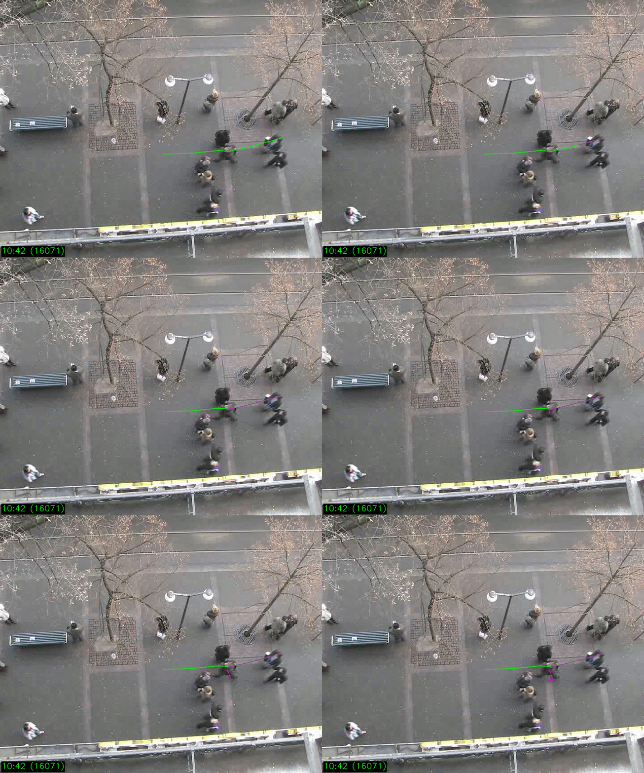
Predicting 4 steps ahead ($T_{pred}=4$), observing 4 steps ($T_{obs}=4$) we obtain 563 trajectories in total with an average mean suqared error of 0.088. We then visualise the result in the following plot.

As you can see the result (in purple) matches the real trajectory (in green) for the first 4 steps since we observed them. However, the followed up predictions (except the first, direct one) do not do as well. The reason for this is that the distribution from which each step is sampled is conditioned on the previously predicted position. Thus, the accumulated error is itself multplicative and leads to such poor behaviour. A few ways to fix this is by iteratively computing each trajectory ignoring the empty steps, by providing more training data or providing more meaningful inputs. Iteratively computing each trajectory together with the rest of the trajectories from the same frame sequence is a relatively simple work around that deems a lot better solutiuons. Motion is conditioned on the surrounding trajectories and optimising each of them along with its neighbours makes a lot of sense. Tutorial 2 from this post’s GitHub repository shows one way of reducing the error exponentially by following this simple trick.

Conclusion

The problem of trajectory modelling is relatively old. Principalled approaches prior to the utilisation of neural solutions use Kalman filters, social utility functions [10] and factorised, interactive Gaussian processes [11]. Albeit the accuracy of some of them, they all assume a lot more prior knowledge prior to modelling the trajectories. Utilising LSTMs, however, extracts the behaviour entirely from data which can be extremely useful in cases where such inductive information is not present. However, it requires larger amounts of data.

One potential way to improve the associated results is by utilising rough inductive biases, ideally extracted in an unsupervised manner. This way, we can ensure a more informed representation that is conditioned on some improtant to each dataset information. One example is utilising both spatial and global dynamics to improve the discussed previously in this blog post representations. Spatial representations would extract static information that is inherent to the given dataset, such as existing trees, surrounding snow etc. While global dynamics deals with modelling the unspoken rules for motion such as the general direction of motion, the way of surpassing individual agents or places agents tend to stay in place, such as at bus stops when waiting for the next bus. [6] models the global social dynamics between agents while [12] utilises both spatial and global dynamics by imputing to features extracted in an unsupervised way. The webpage associated with [12] provides a summary on one way for incorporating inductive biases in a modular way which preserves the small data requirements.

As a quick step towards improving the results we can optimise batches of random sequences of frames instead of optimising batches of random agents. Intuitively, we would like to make sure that we will optimise all agents who are moving alongside together which would essentially consist of a more accurate approximation of the considered data. Further, we will optimise each agent individually and discard all empty slots and apply a few other small tricks. More information can be found in the associated notebook called Tutorial 2. A sample from the resulted solution can be seen bellow.

References

[1] Hochreiter, S. and Schmidhuber, J., 1997. Long short-term memory. Neural computation, 9(8), pp.1735–1780. [2] Graves, A., Mohamed, A.R. and Hinton, G., 2013, May. Speech recognition with deep recurrent neural networks. In Acoustics, speech and signal processing (icassp), 2013 ieee international conference on (pp. 6645–6649). IEEE.

[3] Bowman, S.R., Gauthier, J., Rastogi, A., Gupta, R., Manning, C.D. and Potts, C., 2016. A fast unified model for parsing and sentence understanding. arXiv preprint arXiv:1603.06021.

[4] Sutskever, I., Vinyals, O. and Le, Q.V., 2014. Sequence to sequence learning with neural networks. In Advances in neural information processing systems (pp. 3104–3112).

[5] Yücel, Z., Zanlungo, F., Ikeda, T., Miyashita, T. and Hagita, N., 2013. Deciphering the crowd: Modeling and identification of pedestrian group motion. Sensors, 13(1), pp.875–897.

[6] Alahi, A., Goel, K., Ramanathan, V., Robicquet, A., Fei-Fei, L. and Savarese, S., 2016. Social lstm: Human trajectory prediction in crowded spaces. In Proceedings of the IEEE Conference on Computer Vision and Pattern Recognition (pp. 961–971).

[7] Lerner, A., Chrysanthou, Y. and Lischinski, D., 2007, September. Crowds by example. In Computer Graphics Forum (Vol. 26, №3, pp. 655–664). Oxford, UK: Blackwell Publishing Ltd.

[8] Graves, A., 2013. Generating sequences with recurrent neural networks. arXiv preprint arXiv:1308.0850.

[9] Kingma, D. P., & Ba, J. L. (2015). Adam: a Method for Stochastic Optimization. International Conference on Learning Representations, 1–13.

[10] Yamaguchi, K., Berg, A.C., Ortiz, L.E. and Berg, T.L., 2011, June. Who are you with and where are you going?. In Computer Vision and Pattern Recognition (CVPR), 2011 IEEE Conference on(pp. 1345–1352). IEEE.

[11] Trautman, P. and Krause, A., 2010, October. Unfreezing the robot: Navigation in dense, interacting crowds. In Intelligent Robots and Systems (IROS), 2010 IEEE/RSJ International Conference on (pp. 797–803).

[12] Davchev, T., Burke, M. and Ramamoorthy, S., 2019. Learning Modular Representations for Long-Term Multi-Agent Motion Predictions. arXiv preprint arXiv:1911.13044.