In this blog’s experiments we will utilise the mentioned in previous posts (x,y) coordinate representations as input to the network. Since each of these coordinate representations is associated with a specific agent who will interact with each other, it is important to separate the associated sequences and acknowledge that each prediction will be dependent on the previous sequences observed for a given agent.

Methodology - Stochastic LSTMs

Implementation Details

As we already mentioned, we assume a good understanding of LSTMs. As input to the network we use a sequence of positions of a given agent and each step will be converted to a 128 dimensional feature vector. This conversion happens through a linear operation and a nonlinear, ReLU (Rectified Linear Output) activation.

def embed_inputs(self, inputs, embedding_w, embedding_b):
  # embed the inputs
  with tf.name_scope("Embed_inputs"):
    embedded_inputs = []
    for x in inputs:
        # Each x is a 2D tensor of size numPoints x 2
        embedded_x = tf.nn.relu(tf.add(tf.matmul(x, embedding_w), embedding_b))
        embedded_inputs.append(embedded_x)

    return embedded_inputs

Now that we have a relatively good representation of the input we can feed it through the LSTM model. To do this, we will use 128 dimensional hidden cell state. We chose the hyperparameterisation proposed in [6], [12] where the authors chose them using cross-validation applied on a syntetic dataset. We use learning rate of 0.003, with annealing term of 0.95 and use RMS-prop [5] and L2 regularisation with $\lambda=0.5$ and clip our gradients between -10 and 10.

NUM_EPOCHS = 100
DECAY_RATE = 0.95
GRAD_CLIP = 10
LR = 0.003
NUM_UNITS = 128
EMBEDDING = 128
MODE = 'train'

SAVE_PATH='save'

avg_time = 0 # used for printing
avg_loss = 0 # used for printing

We achieve this task by updating the associated with the LSTM cell state at each step as follows:

def lstm_advance(self, embedded_inputs, cell, scope_name="LSTM"):
  # advance the lstm cell state with one for each entry
  with tf.variable_scope(scope_name) as scope:
    state = self.initial_state
    outputs = []
    for i, inp in enumerate(embedded_inputs):
      if i > 0:
        scope.reuse_variables()
      output, last_state = cell(inp, state)
      outputs.append(output)
 
    return outputs, last_state

Having done this, we can now convert the output from the LSTM in a 5 dimensional output.

def final_layer(self, outputs, output_w, output_b):
  with tf.name_scope("Final_layer"):
    # Apply the linear layer. Output would be a 
    # tensor of shape 1 x output_size
    output = tf.reshape(tf.concat(outputs, 1), [-1, self.num_units])
    output = tf.nn.xw_plus_b(output, output_w, output_b)
    return output

We will use this output to define the distribution we will sample a predicted position $y_t$ and namely a 2D Gaussian distribution with a mean value $\mu = [\mu_x, \mu_y]$, standard deviation $\sigma = [\sigma_x, \sigma_y]$ and correlation $\rho$, similar to the described approach in [8].

Please note that these $x_t$ and $y_t$ are different from the $(x,y)$ coordinates. In this case, $(x, y)_t$ represent input and output to the proposed model at time $t$. We indicate the output of the proposed model as $\hat{y_t}$ and namely:

In this case, $b_y$ is the associated bias, $W$ are the parameters of the last layer’s feedforward layer and $h$ are the hidden output parameters from the LSTM. We ensure that the output representing the standard deviation will always be positive by representing the output of the network using an exponential function and ensure that the correlation term will be scaled between -1 and 1 using $tanh$.

We can then define the probability $p(x_{t+1}\vert y_y)$ utilising the previous target $y_t$ can be defined as:

$p(x_{t+1} \vert y_y) = N(x_{t+1} \vert \mu_t, \sigma_t, \rho_t)$, for $N(x \vert \mu, \sigma, \rho) = {1\over{2\pi\sigma_1\sigma_2\sqrt{1-\rho^2}}}exp\big{[}{-Z\over{2(1-\rho^2})}\big{]}$, with

.

With this we obtain a loss function which is exact to a constant and depends entirely on the quantisation of the actual information and is in no way affecting the training of the network.

$\mathcal{L} = \sum^T_{t=1}-log\big{(}N(x_{t+1} \vert \mu_t, \sigma_t, \rho_t)\big{)}$

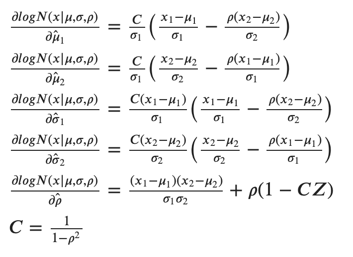
Further, we can extract the partial derivatives for the five components and obtain:

As code, we can implement the associated loss function with the following 2 functions:

def get_lossfunc(g, z_mux, z_muy, z_sx, z_sy, z_corr, x_data, y_data):
  # Calculate the PDF of the data w.r.t to the distribution
  result0 = \
    distributions.tf_2d_normal(g, x_data, y_data, z_mux, z_muy, z_sx, z_sy, z_corr)

  # For numerical stability purposes as in Vemula (2018)
  epsilon = 1e-20

  # Numerical stability
  result1 = -tf.log(tf.maximum(result0, epsilon))

  return tf.reduce_sum(result1)

def tf_2d_normal(g, x, y, mux, muy, sx, sy, rho):
  '''
  Function that computes a multivariate Gaussian
  Equation taken from 24 & 25 in Graves (2013)
  '''
  with g.as_default():
    # Calculate (x-mux) and (y-muy)
    normx = tf.subtract(x, mux)
    normy = tf.subtract(y, muy)
    # Calculate sx*sy
    sxsy = tf.multiply(sx, sy)
    # Calculate the exponential factor
    z = tf.square(tf.divide(normx, sx)) + \
        tf.square(tf.divide(normy, sy)) - \
        2*tf.divide(
          tf.multiply(rho, tf.multiply(normx, normy)),
          sxsy)
  
    negatedRho = 1 - tf.square(rho)
    # Numerator
    result = tf.exp(tf.divide(-z, 2*negatedRho))
    # Normalization constant
    denominator = \
      2 * np.pi * tf.multiply(sxsy, tf.sqrt(negatedRho))
  
    # Final PDF calculation
    result = tf.divide(result, denominator)

    return result

To our convenience, Tensorflow is capable of computing the derivatives automatically and we do not need to worry about implementing this bit. All that is left is to choose the optimisation routine.

As previously mentioned, we will use L2 regularisation since we want to enforce a single optimsal solution (namely the targeted positions $y_t$). This way we constrain the accuracy during training (or the potential to overfit) by ensuring better generalisation achieved via efficient (in terms of compute) approach. In addition, we clip our gradients between 10 and -10 and ensure we will not face problems associated with exploding gradients. Finally, we will use RMS-Prop, an unpublished optimisation algorithm. The algorithm is famous for using the second moment representing the variation of the previous gradient squared. As an alternative, we can use Adam [9] which normalises the gradients using first and second moment which also corrects for the bias during training. However, empirically, we found RMS-Prop to work better in this task. We hypothesise that this could be due the fact that we are interested in exploiting some of the biases of motion as we do not aim to generalise to other agents than human beings. You can find out more about different optimisation algorithms in S. Ruder’s blog post.

if self.mode != tf.contrib.learn.ModeKeys.INFER:
  with tf.name_scope("Optimization"):
    lossfunc = self.get_lossfunc(o_mux, o_muy, o_sx, o_sy, o_corr, x_data, y_data)

    self.cost = tf.div(lossfunc, (self.batch_size * self.sequence_length))
    trainable_params = tf.trainable_variables()

    # apply L2 regularisation
    l2 = 0.05 * sum(tf.nn.l2_loss(t_param) for t_param in trainable_params)
    self.cost = self.cost + l2
    tf.summary.scalar('cost', self.cost)

    self.gradients = tf.gradients(self.cost, trainable_params)
    grads, _ = tf.clip_by_global_norm(self.gradients, self.grad_clip

    # Adam might also do a good job as in Graves (2013)
    optimizer = tf.train.RMSPropOptimizer(self.lr)
    # Train operator
    self.train_op = optimizer.apply_gradients(zip(grads, trainable_params))

    self.init = tf.global_variables_initializer()

Finally, we can define the entire model as shown in the section below.

reset_graph()
lstm = BasicLSTM(batch_size=BATCH_SIZE,
                 sequence_length=SEQUENCE_LENGTH,
                 num_units=NUM_UNITS,
                 embedding_size=EMBEDDING,
                 learning_rate=LR,
                 grad_clip=GRAD_CLIP,
                 mode=MODE)